DAX Formulae For Creating Statistical Distributions in Power BI
Here I share the DAX code for creating various statistical distributions in Power BI


As a simulation engineer, one of my responsibilities is to create statistical experiments to simulate various scenarios and understand the outcomes. These outcomes have probabilities associated with them which help the decision makers to identify key risks, uncertainties and make informed decisions to leverage risk. For example, if the company wants to invest a million dollars in a capital project, there are many uncertainties involved such as labor costs, scheduling uncertainty, project delays, technical risks etc. A statistical simulation experiment, i.e Monte Carlo simulation, will assign probabilities with these risks and simulate thousands of outcomes to compute the probability of success. The company can then decide if it wants to invest the $1M or what decisions it can take proactively to de-risk the uncertainties.
There are many statistical packages and Excel add-ons available to create such experiments but none that I know of in Power BI. In Power BI, only uniform distribution and normal distributions are available natively in DAX. In this blog post I share the DAX codes I use to create different distibutions.
If you are new to Monte Carlo / Discrete Event simulation, these distributions may not make sense. In a future blog post I will show when to use these distributions and how to create sophisticated simulations in Power BI. The beauty of creating it in Power BI vs Excel is that the stakeholders can interact with the simulation parameters and understand the probable outcomes much more clearly. The DAX codes given here can be used to create calculated tables for simulations.
If you are interested in this topic, please also take a look at my other blog on generating random numbers in Power BI


LogNormal Distribution
LogNormal distribution with mean = 80, variance = 225
DAX:
LogNormal =

VAR _m = 80 // mean
VAR _v = 225 // variance (not std deviation)
VAR _phi =
SQRT ( _v + _m ^ 2 )
VAR _mu =
    LN ( ( _m ^ 2 ) / _phi ) // scaled mean
VAR _sigma =
SQRT ( LN ( ( _phi ^ 2 ) / _m ^ 2 ) )
RETURN

// scaled s.d

EXP ( NORM.INV ( RAND (), _mu, _sigma ) )
Beta PERT
Beta PERT with: Min likely value = 100 Med likely value = 300 Max likely value = 800
DAX:
Beta Pert =

VAR _a = 100
VAR _b = 300
VAR _c = 800
VAR _alpha = ( 4 * _b + _c - 5 * _a ) / ( _c - _a )
VAR _beta = ( 5 * _c - _a - 4 * _b ) / ( _c - _a )
RETURN
    BETA.INV ( RAND (), _alpha, _beta, _a, _c )
Discrete
Discrete with:
Probability of Choice 1 = 50% , Probability of Choice 2 = 30% , Probability of Choice 3 = 20%
DAX:
Discrete =
IF (
    'Table'[random_chocie] <= 0.5,
    "Choice 1",
    IF (
         ( 'Table'[random_chocie] > 0.5
            && 'Table'[random_chocie] < 0.8 ),
        "Choice 2",
        IF ( ( 'Table'[random_chocie] > 0.8 ), "Choice 3" )
    )
)


Truncated Normal Distribution
Truncated normal distribution with: lower limit = 1 higher limit = 4 mean = 3 s.d = 0.9
DAX: truncatednormal =
VAR _a = 1
VAR _b = 4
VAR _mu = 3
VAR _sigma = 0.9
RETURN
    NORM.INV (
        NORM.DIST ( _a, _mu, _sigma, TRUE )
            + RAND ()
                * (
                    NORM.DIST ( _b, _mu, _sigma, TRUE )
                        - NORM.DIST ( _a, _mu, _sigma, TRUE )
                ),
        _mu,
        _sigma
    )


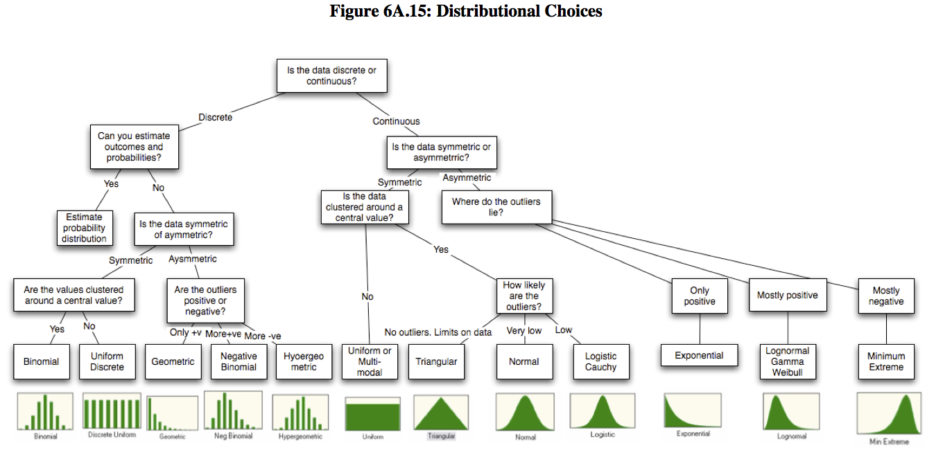
You may find below visual helpful in determining which distribution to use: