Penalized Linear Regression in Azure ML Studio Designer
Using Ridge regression with L2 norm penalty to improve OLS linear regression in Azure ML Studio


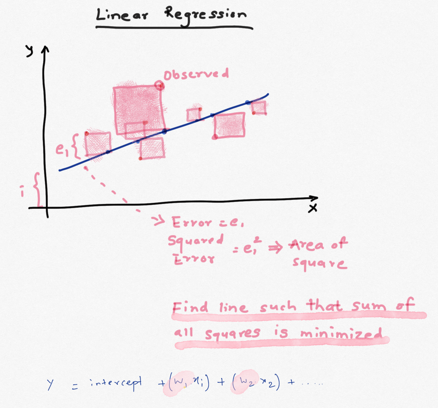
Linear Regression
Linear regression is the simplest and the most basic form of regression. Many textbooks and videos cover it in detail. To predict an outcome y using features x1,x2,x3..., we take a weighted sum of all the features (plus an intercept term). The weight assigned to each feature is obtained by minimizing the sum of squared errors (SSE). The larger the weight, the higher it contributes to predicting y. The main advantages of using linear regression are that it is fairly easy to interprete, model and doesn't require lot of data. The drawbacks are that it requires features to be uncorrelated, features need to be numerical, model often underfits the data and it cannot be used for complex non-linear relationships. If the feautures are correlated they can reduce the accuracy of the predictions and results become less interpretable.
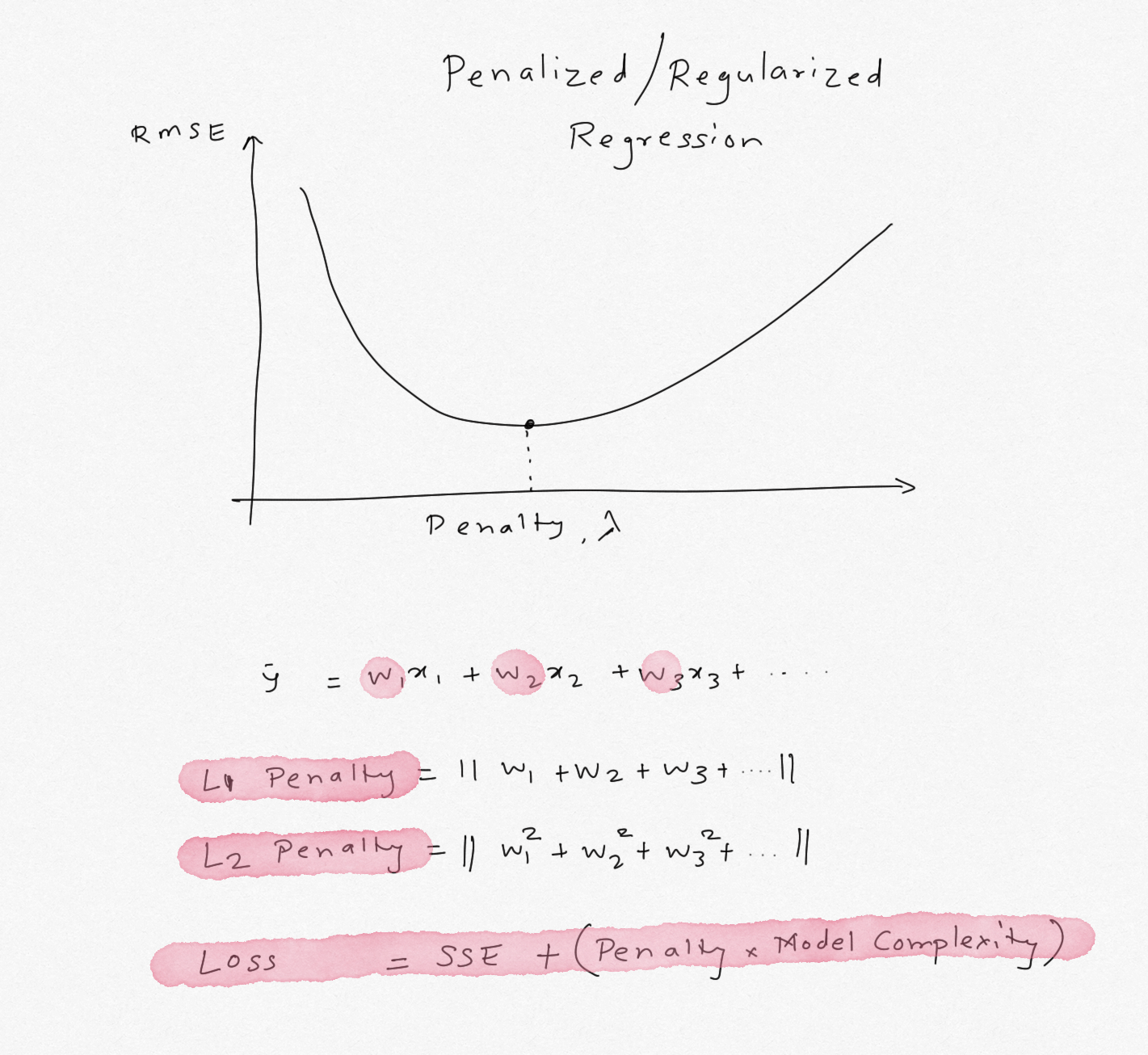
The weights calculated using the min(SSE) criterion have high bias and low variance. We can fix this by adding more non-linear additive terms, thereby increasing the bias but lowering the variance. As the model becomes relatively more complex, the weights obtained for these features also increase and can lead to larger variance. To tackle this problem, a penalty term is added to SSE that penalizes the features that have large weights. If the penalty is 0, resulting model is just OLS but as the penalty increases, the weights have to shrink to satisfy min(SSE) criterion. As the weights become very large, they almost shrink to zero. If we can identify the right penalty, we can achieve lower variance sacrificing bias. Such model will generalize better and will be less susciptible to effects from multicollinear features.
The penalty can be assigned to the absolute sum of the weights (L1 norm) or sum of squared weights (L2 norm). Linear regression using L1 norm is called Lasso Regression and regression with L2 norm is called Ridge Regression.
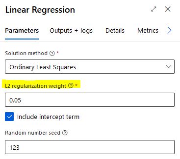
Azure ML Studio offers Ridge regression with default penalty of 0.001. As mentioned above, if the penalty is small, it becomes OLS Linear Regression. This penalty can be adjusted to implement Ridge Regression. Typically the penalty is calculated using k-fold cross-validation for a range of penalty values either by random search or grid search. Unfortunately Azure ML Studio does not offer parameter sweep / grid search for tuning the L2 penalty in the Studio, so we will have to find the optimal penalty in the notebook and use it in the designer. Note that the penalty depends on the data, so if the data change significantly, the value will have to be re-calculated. As the penalty increases, bias increases but variance reduces (because model complexity reduces due to penalty on weights) and after an optimal value of the penalty, variance increases again.
#collapse-hide
import pandas as pd
from sklearn.preprocessing import OneHotEncoder, LabelEncoder, StandardScaler, QuantileTransformer, Normalizer, PowerTransformer
from sklearn.linear_model import LinearRegression, Ridge, RidgeCV, Lasso, LassoCV, ElasticNet, ElasticNetCV
from sklearn.metrics import mean_absolute_error, r2_score, mean_squared_error
from sklearn.model_selection import train_test_split, cross_validate, cross_val_score
from sklearn.pipeline import make_pipeline, Pipeline
from sklearn.compose import ColumnTransformer
from statsmodels.tools.eval_measures import rmse
from sklearn.ensemble import RandomForestRegressor
from sklearn.tree import DecisionTreeClassifier, DecisionTreeRegressor
import numpy as np
import seaborn as sns
import matplotlib.pyplot as plt
%matplotlib inline
import warnings
warnings.filterwarnings('ignore')
from nimbusml.linear_model import FastLinearRegressor
#collapse-hide
def corr_heatmap (df, target = 'Salary',threshold = 0.5 ,annot = False, absolute = False):
    '''
    Sandeep Pawar
    Create a triangular correlation plot and highlight strong correlations based on specified threshold
    import seaborn as sns

    '''
    plt.figure(figsize=(12,9))
    mask = np.triu(np.ones_like(df.corr(), dtype=np.bool))
    cmap = sns.diverging_palette(220, 20, n=10, sep = 80)

    if absolute == True:
        df = df.corr().abs().round(1).sort_values(by=target)
    else:
        df = df.corr().round(1).sort_values(by=target)

    sns.heatmap(df,
                annot=annot,
                cmap=cmap,
                mask=mask ,
                vmax = threshold,
                center = 0,
                vmin = -threshold,
                square = True);
Data
I am going to use data of baseball hitters. The data has stats for each player and their salary. The goal is to predict a player's salary using their stats. This data has 3 categorical features and 16 numerical features. I have dropped the player's name from the data.
path = "https://gist.githubusercontent.com/keeganhines/59974f1ebef97bbaa44fb19143f90bad/raw/d9bcf657f97201394a59fffd801c44347eb7e28d/Hitters.csv"

df = (pd.read_csv(path).dropna().drop("Unnamed: 0",axis=1) )

categoricals = ['League','Division','NewLeague']

numericals = ['AtBat', 'Hits', 'HmRun', 'Runs', 'RBI', 'Walks', 'Years', 'CAtBat', 'CHits', 'CHmRun', 'CRuns', 'CRBI', 'CWalks','PutOuts', 'Assists', 'Errors' ]

df[categoricals]=df[categoricals].astype('category')

df.head(3)
I won't spend much time here on EDA as the purpose is to show how to implement penalized regression in Azure mL Studio. But as the correlation matrix below shows, the features show very high collinearity with each other but moderate correlation with the target variable Salary.
I will include all the features in the model to show how Ridge Regression improves the results of Linear Regression despite highly correlated features.
corr_heatmap(df, threshold = 0.9, absolute=False, annot=True, target ='Salary')

Above heatmap shows, many features are highly correlated with each other and have low-medium correlation with the target variable Salary.
#Creating train test split with 20% test

X = df.drop('Salary', axis=1)
y = df['Salary'].values


x1,x2,y1,y2 = train_test_split(X,y,test_size=0.2, random_state=123 )
print("Train Size:",len(x1))
print("RTest Size:",len(x2))
Scikit-Learn
For linear regression, all the features need to be numericals and need to be scaled. While scaling is not a requirement, for Ridge Regression the features should be scaled to make sure feature scales don't influence the weights. Categorical features will be one-hot encoded and numerical features will be scaled using StandardScaler().
#Create a quick pipeline


cat_ohe = OneHotEncoder()
cat_steps = [('OHE', cat_ohe)]
cat_pipe = Pipeline(cat_steps)

ss=StandardScaler()
num_steps = [('Scaler', ss)]
num_pipe = Pipeline(num_steps)

transformers = [('Categoricals', cat_pipe, categoricals),
                ('Numericals', num_pipe, numericals)]

ct = ColumnTransformer(transformers)

x1_scaled = ct.fit_transform(x1)
x2_scaled = ct.transform(x2)

#Linear Regression
lr = LinearRegression()
steps = [('Transform', ct),('LinearRegression', lr)]
pipe_final = Pipeline(steps)
pipe_final.fit(x1,y1)

print("OLS Train RMSE:",rmse(y1,pipe_final.predict(x1)))
print("OLS Test RMSE:",rmse(y2,pipe_final.predict(x2)))
print("------------------------------------")

#Ridge Regression
rr = Ridge(alpha=402)
rr.fit(x1_scaled,y1)
rr.predict(x2_scaled)

print("Ridge Train RMSE:",rmse(y1,rr.predict(x1_scaled)))
print("Ridge Test RMSE:",rmse(y2,rr.predict(x2_scaled)))
print("------------------------------------")

#Lasso Regression
lasso = Lasso(alpha=15)
lasso.fit(x1_scaled,y1)
lasso.predict(x2_scaled)

print("Lasso Train RMSE:",rmse(y1,lasso.predict(x1_scaled)))
print("Lasso Test RMSE:",rmse(y2,lasso.predict(x2_scaled)))
print("------------------------------------")

#Decision Tree
dt = DecisionTreeRegressor(random_state=123, max_depth=3, min_samples_leaf=0.10)
dt.fit(X=x1_scaled,y=y1)
dt.predict(x2_scaled)

print("DT Train RMSE:",rmse(y1,dt.predict(x1_scaled)))
print("DT Test RMSE:",rmse(y2,dt.predict(x2_scaled)))
print("------------------------------------")

#Random Forest
rf = RandomForestRegressor()
rf.fit(X=x1_scaled,y=y1)
rf.predict(x2_scaled)

print("RF Train RMSE:",rmse(y1,rf.predict(x1_scaled)))
print("RF Test RMSE:",rmse(y2,rf.predict(x2_scaled)))
As the results show, with Linear Regression, RMSE is 300 and 388 on train & test, resp. With Ridge Regression, I tuned the parameter to alpha=402 and obtained RMSE of 342/327. Thus using Ridge regression, the RMSE on training set increased (higher bias) but the RMSE on test set decreased (lower variance). In comparison, Lasso Regression was slightly worse than Ridge regression. Decision Tree and Random Forest were significantly better without tuning any parameters !
coef=pd.DataFrame()
n = list(np.arange(len(rr.coef_)))
for i in n:
    coef=coef.append({"Feature":i,
                      "Linear Reg":lr.coef_[i],
                      "Ridge Reg":rr.coef_[i],
                      "Lasso Reg": lasso.coef_[i]},ignore_index=True)
coef.set_index('Feature').sort_values(by='Ridge Reg', ascending=False).plot.bar(grid=False, figsize=(15,8));

The chart and table above show weight on each feature used to train the model. In all cases, the weights have decreased with Ridge Regression compared to Linear Regression. That's the effect of using a high penalty. In comparison, Lasso regresion shrinks the weights to exactly zero for some of the features. Lasso has an advantage of feature selection. Out of the 21 features used, only 8 features have non-zero weights and are important for predicting the outcome!
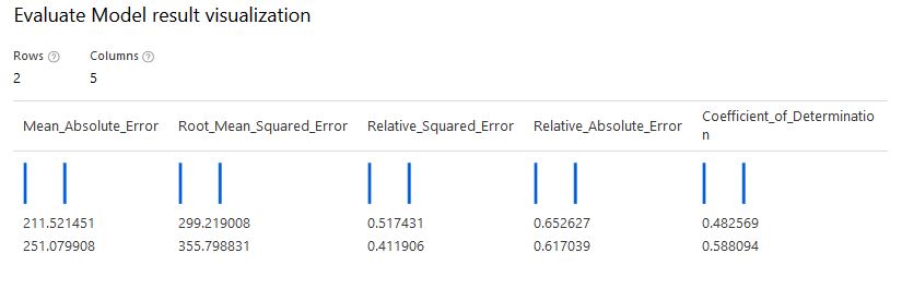
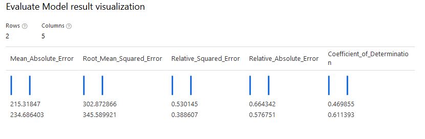
In Azure ML designer the L2 penalty did not produce same results despite using the same data and parameters. I suspected that this is because Azure ML Studio uses the FastLinearRegressor() instead of Ridge() from scikit-learn. So I tuned the parameters using FastLinearRegressor() from nimbusml. The optimal L2 was 0.04 to 0.06. This showed improvement over the OLS Regression in AzureML Studio. RMSE over test set dropped from 355 to 345. Not a significant drop but if linear regresison is needed, Ridge will generalize better than Linear Regression.
My take-aways are :
- Azure ML Studio offers Ridge Regression which can provide better results over Linear Regression when features have multi-collinearity
- Azure ML Studio does not offer tuning or grid-searching the L2 penalty. This has to be done either by running multiple experiments in the Studio or in external notebook.
-
FastLinearRegressor()does not offer Lasso Regression directly but by adjusting thel1_thresholdparameter we can run Lasso or ElasticNet Regression. This will achieve a compromise between Lasso and Ridge. Lasso or ElasticNet are not available in the Studio. - By default
FastLinearRegressor()normalizes the data, it's not clear from the documentation if thats the default behaviour in Studio when L2 penalty is used. - The hyperparameters tuned in sklearn do not directly work in Studio. Be sure tune them in Studio.